Examples

Create Fit with LocalPolynomialRegression

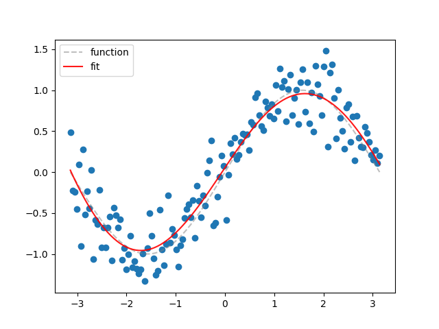
Use the method LocalPolynomialRegression.fit in order to create the fit for the dataset and estimate the first and second derivative for the fit:

import numpy as np
from matplotlib import pyplot as plt
from localpoly.base import LocalPolynomialRegression

np.random.seed(1)
X = np.linspace(-np.pi, np.pi, num=150)
y_real = np.sin(X)
y = np.random.normal(0, 0.3, len(X)) + y_real

model = LocalPolynomialRegression(X=X, y=y, h=0.8469, kernel="gaussian", gridsize=100)
prediction_interval = (X.min(), X.max())
results = model.fit(prediction_interval)

plt.scatter(X, y)
plt.plot(X, y_real, "grey", ls="--", alpha=0.5, label="function")
plt.plot(results["X"], results["fit"], "r", alpha=0.9, label="fit")
plt.legend()
plt.show()

Bandwidth Optimization with LocalPolynomialRegressionCV

Use the method LocalPolynomialRegressionCV.bandwidth_cv in order to optimize the bandwidth for the selected kernel:

import numpy as np
from matplotlib import pyplot as plt
from localpoly.base import LocalPolynomialRegressionCV

np.random.seed(1)
X = np.linspace(-np.pi, np.pi, num=150)
y_real = np.sin(X)
y = np.random.normal(0, 0.3, len(X)) + y_real

model_cv = LocalPolynomialRegressionCV(
    X=X,
    y=y,
    kernel="gaussian",
    n_sections=15,
    loss="MSE",
    sampling="random",
)

results = model_cv.bandwidth_cv(np.linspace(0.5, 1.0, 10))
print(f"Optimal bandwidth: {results['fine results']['h']}")
plt.plot(results["coarse results"]["bandwidths"], results["coarse results"]["MSE"])
plt.plot(results["fine results"]["bandwidths"], results["fine results"]["MSE"])
plt.show()